# Yeast program, to study growth of yeast using Euler's method
# First, specify the starting and ending points, stepsize, and total number of observation points
tstart=0
tfin=60
stepsize=0.1
length=(tfin-tstart)/stepsize+1
# Next, specify the intial amount of yeast Y; alcohol A; the carrying capacity b; the toxicity coefficient c; and the growth rate k
Y=0.5
A=0
b=10
c=0.1
k=0.2
t=tstart
# Next we create lists to store our computed values of t, A and Y
Yvalues=[]
Avalues=[]
tvalues=[]
# The following loop does three things:
# (1) stores the current values of Y and t into the lists created above;
# (2) computes the next value of Y using Euler's method;
# (3) increases t by the stepsize
for i in range(length):
# Store current values of Y, A, and t
Yvalues.append(Y)
Avalues.append(A)
tvalues.append(t)
# Compute rate of change using logistic equation and appropriate rate equation
Yprime=k*Y*(1-Y/b)-c*A*Y
Aprime=.05*Y
# Net change equals rate of change times stepsize, for Y and A
DeltaY=Yprime*stepsize
DeltaA=Aprime*stepsize
# New values equal current values plus net change, for Y, A, and t
Y=Y+DeltaY
A=A+DeltaA
t=t+stepsize
# Next time through the loop, the above new values play the role of current values
# Zip the t values with the S/I/R values into lists of ordered pairs, and create plots of these
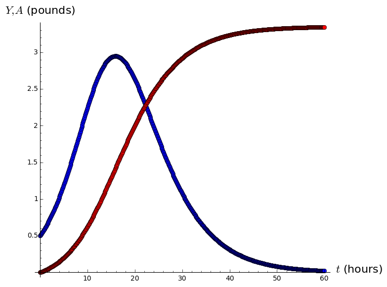
Yplot=list_plot(list(zip(tvalues,Yvalues)),plotjoined=True,marker='o',color='blue')
Aplot=list_plot(list(zip(tvalues,Avalues)),plotjoined=True,marker='o',color='red')
# Now plot the computed Y and A values against the corresponding points in the domain
show(Yplot+Aplot,axes_labels=['$t$ (hours)','$Y,A$ (pounds)'])
|
# Yeast program, to study growth of yeast using Euler's method
# First, specify the starting and ending points, stepsize, and total number of observation points
tstart=0
tfin=60
stepsize=0.1
length=(tfin-tstart)/stepsize+1
# Next, specify the intial amount of yeast Y; alcohol A; sugar S; the carrying capacity b; the toxicity coefficient c; and the growth rate k
Y=0.5
A=0
S=25
b=.4
c=0.1
k=0.2
t=tstart
# Next we create lists to store our computed values of t, A S, and Y
Yvalues=[]
Avalues=[]
Svalues=[]
tvalues=[]
# The following loop does three things:
# (1) stores the current values of Y and t into the lists created above;
# (2) computes the next value of Y using Euler's method;
# (3) increases t by the stepsize
for i in range(length):
# Store current values of Y, A, S, and t
Yvalues.append(Y)
Avalues.append(A)
Svalues.append(S)
tvalues.append(t)
# Compute rate of change using logistic equation and appropriate rate equation
Yprime=k*Y*(1-Y/(b*S))-c*A*Y
Aprime=.05*Y
Sprime=-0.15*Y
# Net change equals rate of change times stepsize, for Y, S and A
DeltaY=Yprime*stepsize
DeltaA=Aprime*stepsize
DeltaS=Sprime*stepsize
# New values equal current values plus net change, for Y, A, S, and t
Y=Y+DeltaY
A=A+DeltaA
S=S+DeltaS
t=t+stepsize
# Next time through the loop, the above new values play the role of current values
# Zip the t values with the S/I/R values into lists of ordered pairs, and create plots of these
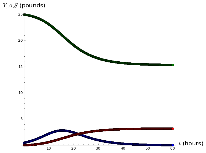
Yplot=list_plot(list(zip(tvalues,Yvalues)),plotjoined=True,marker='o',color='blue')
Aplot=list_plot(list(zip(tvalues,Avalues)),plotjoined=True,marker='o',color='red')
Splot=list_plot(list(zip(tvalues,Svalues)),plotjoined=True,marker='o',color='green')
# Now plot the computed Y, S and A values against the corresponding points in the domain
show(Yplot+Aplot+Splot,axes_labels=['$t$ (hours)','$Y,A,S$ (pounds)'])
|
|
|