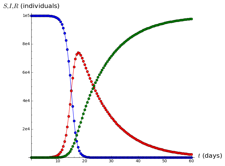
# First, specify the starting and ending points, stepsize, and total number of observation points
tstart=0
tfin=60
stepsize=0.5
length=(tfin-tstart)/stepsize+1
# Next, specify values of parameters, and initial values of variables
a=0.00001
b=1/12
S=99999
I=1
R=0
t=tstart
# Set up empty lists for the values we're about to compute
Svalues=[]
Ivalues=[]
Rvalues=[]
tvalues=[]
# The following loop does three things:
# (1) stores the current values of S, I, R, and t into the lists created above;
# (2) computes the next values of S, I, R using Euler's method;
# (3) increases t by the stepsize
for i in range(length):
# Store current values
Svalues.append(S)
Ivalues.append(I)
Rvalues.append(R)
tvalues.append(t)
# Compute rates of change using SIR equations
Sprime=-a*S*I
Iprime=a*S*I-b*I
Rprime=b*I
# Net change equals rate of change times stepsize
DeltaS=Sprime*stepsize
DeltaI=Iprime*stepsize
DeltaR=Rprime*stepsize
# New values equal current values plus net change
S=S+DeltaS
I=I+DeltaI
R=R+DeltaR
t=t+stepsize
# Next time through the loop, the above new values play the role of current values
# Zip the t values with the S/I/R values into lists of ordered pairs, and create plots of these
A=list_plot(list(zip(tvalues,Svalues)),plotjoined=True,marker='o',color='blue')
B=list_plot(list(zip(tvalues,Ivalues)),plotjoined=True,marker='o',color='red')
C=list_plot(list(zip(tvalues,Rvalues)),plotjoined=True,marker='o',color='green',axes_labels=['$t$ (days)','$S,I,R$ (individuals)'])
SIRgraph=A+B+C
show(SIRgraph)
|
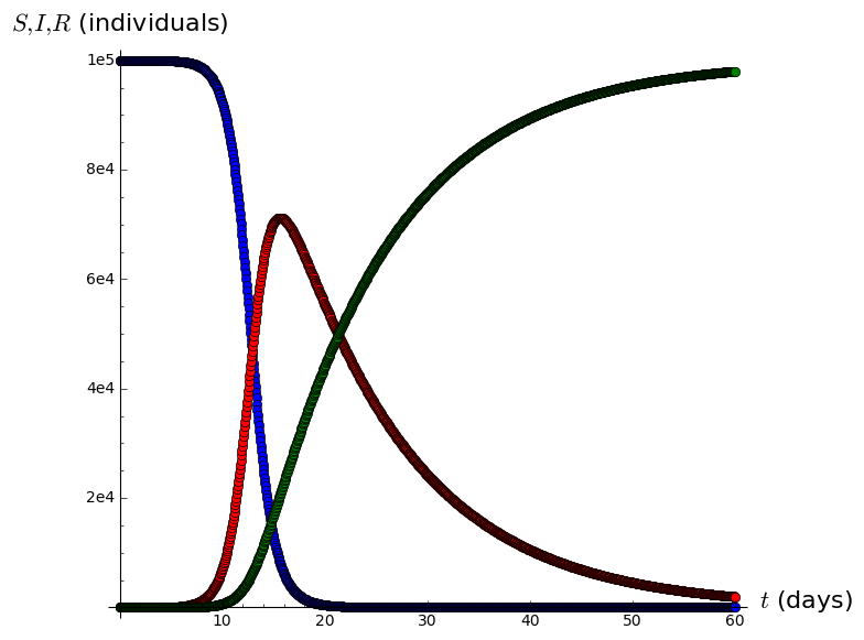
# First, specify the starting and ending points, stepsize, and total number of observation points
tstart=0
tfin=60
stepsize=0.05
length=(tfin-tstart)/stepsize+1
# Next, specify values of parameters, and initial values of variables
a=0.00001
b=1/12
S=99999
I=1
R=0
t=tstart
# Set up empty lists for the values we're about to compute
Svalues=[]
Ivalues=[]
Rvalues=[]
tvalues=[]
# The following loop does three things:
# (1) stores the current values of S, I, R, and t into the lists created above;
# (2) computes the next values of S, I, R using Euler's method;
# (3) increases t by the stepsize
for i in range(length):
# Store current values
Svalues.append(S)
Ivalues.append(I)
Rvalues.append(R)
tvalues.append(t)
# Compute rates of change using SIR equations
Sprime=-a*S*I
Iprime=a*S*I-b*I
Rprime=b*I
# Net change equals rate of change times stepsize
DeltaS=Sprime*stepsize
DeltaI=Iprime*stepsize
DeltaR=Rprime*stepsize
# New values equal current values plus net change
S=S+DeltaS
I=I+DeltaI
R=R+DeltaR
t=t+stepsize
# Next time through the loop, the above new values play the role of current values
# Zip the t values with the S/I/R values into lists of ordered pairs, and create plots of these
A=list_plot(list(zip(tvalues,Svalues)),plotjoined=True,marker='o',color='blue')
B=list_plot(list(zip(tvalues,Ivalues)),plotjoined=True,marker='o',color='red')
C=list_plot(list(zip(tvalues,Rvalues)),plotjoined=True,marker='o',color='green',axes_labels=['$t$ (days)','$S,I,R$ (individuals)'])
SIRgraph=A+B+C
show(SIRgraph)
|
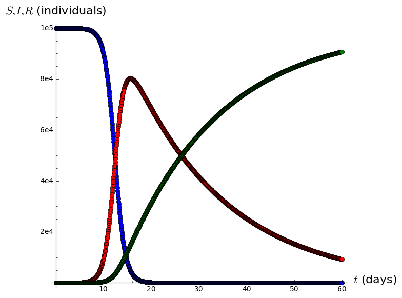
# First, specify the starting and ending points, stepsize, and total number of observation points
tstart=0
tfin=60
stepsize=0.05
length=(tfin-tstart)/stepsize+1
# Next, specify values of parameters, and initial values of variables
a=0.00001
b=1/20
S=99999
I=1
R=0
t=tstart
# Set up empty lists for the values we're about to compute
Svalues=[]
Ivalues=[]
Rvalues=[]
tvalues=[]
# The following loop does three things:
# (1) stores the current values of S, I, R, and t into the lists created above;
# (2) computes the next values of S, I, R using Euler's method;
# (3) increases t by the stepsize
for i in range(length):
# Store current values
Svalues.append(S)
Ivalues.append(I)
Rvalues.append(R)
tvalues.append(t)
# Compute rates of change using SIR equations
Sprime=-a*S*I
Iprime=a*S*I-b*I
Rprime=b*I
# Net change equals rate of change times stepsize
DeltaS=Sprime*stepsize
DeltaI=Iprime*stepsize
DeltaR=Rprime*stepsize
# New values equal current values plus net change
S=S+DeltaS
I=I+DeltaI
R=R+DeltaR
t=t+stepsize
# Next time through the loop, the above new values play the role of current values
# Zip the t values with the S/I/R values into lists of ordered pairs, and create plots of these
A=list_plot(list(zip(tvalues,Svalues)),plotjoined=True,marker='o',color='blue')
B=list_plot(list(zip(tvalues,Ivalues)),plotjoined=True,marker='o',color='red')
C=list_plot(list(zip(tvalues,Rvalues)),plotjoined=True,marker='o',color='green',axes_labels=['$t$ (days)','$S,I,R$ (individuals)'])
SIRgraph=A+B+C
show(SIRgraph)
|
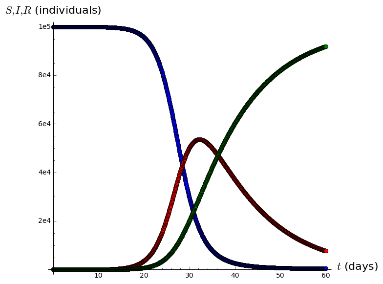
# First, specify the starting and ending points, stepsize, and total number of observation points
tstart=0
tfin=60
stepsize=0.05
length=(tfin-tstart)/stepsize+1
# Next, specify values of parameters, and initial values of variables
a=0.000005
b=1/12
S=99999
I=1
R=0
t=tstart
# Set up empty lists for the values we're about to compute
Svalues=[]
Ivalues=[]
Rvalues=[]
tvalues=[]
# The following loop does three things:
# (1) stores the current values of S, I, R, and t into the lists created above;
# (2) computes the next values of S, I, R using Euler's method;
# (3) increases t by the stepsize
for i in range(length):
# Store current values
Svalues.append(S)
Ivalues.append(I)
Rvalues.append(R)
tvalues.append(t)
# Compute rates of change using SIR equations
Sprime=-a*S*I
Iprime=a*S*I-b*I
Rprime=b*I
# Net change equals rate of change times stepsize
DeltaS=Sprime*stepsize
DeltaI=Iprime*stepsize
DeltaR=Rprime*stepsize
# New values equal current values plus net change
S=S+DeltaS
I=I+DeltaI
R=R+DeltaR
t=t+stepsize
# Next time through the loop, the above new values play the role of current values
# Zip the t values with the S/I/R values into lists of ordered pairs, and create plots of these
A=list_plot(list(zip(tvalues,Svalues)),plotjoined=True,marker='o',color='blue')
B=list_plot(list(zip(tvalues,Ivalues)),plotjoined=True,marker='o',color='red')
C=list_plot(list(zip(tvalues,Rvalues)),plotjoined=True,marker='o',color='green',axes_labels=['$t$ (days)','$S,I,R$ (individuals)'])
SIRgraph=A+B+C
show(SIRgraph)
|
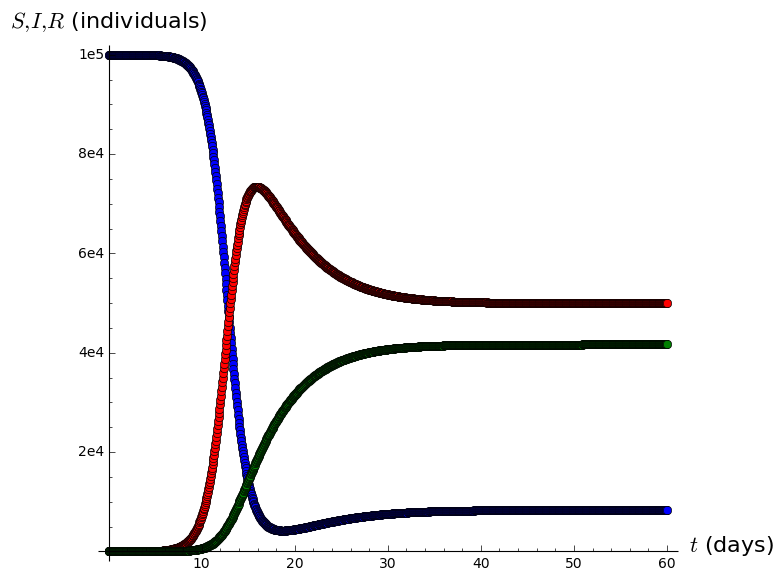
# First, specify the starting and ending points, stepsize, and total number of observation points
tstart=0
tfin=60
stepsize=0.05
length=(tfin-tstart)/stepsize+1
# Next, specify values of parameters, and initial values of variables
a=0.00001
b=1/12
c=10
S=99999
I=1
R=0
t=tstart
# Set up empty lists for the values we're about to compute
Svalues=[]
Ivalues=[]
Rvalues=[]
tvalues=[]
# The following loop does three things:
# (1) stores the current values of S, I, R, and t into the lists created above;
# (2) computes the next values of S, I, R using Euler's method;
# (3) increases t by the stepsize
for i in range(length):
# Store current values
Svalues.append(S)
Ivalues.append(I)
Rvalues.append(R)
tvalues.append(t)
# Compute rates of change using SIR equations
Sprime=-a*S*I+(1/c)*R
Iprime=a*S*I-b*I
Rprime=b*I-(1/c)*R
# Net change equals rate of change times stepsize
DeltaS=Sprime*stepsize
DeltaI=Iprime*stepsize
DeltaR=Rprime*stepsize
# New values equal current values plus net change
S=S+DeltaS
I=I+DeltaI
R=R+DeltaR
t=t+stepsize
# Next time through the loop, the above new values play the role of current values
# Zip the t values with the S/I/R values into lists of ordered pairs, and create plots of these
A=list_plot(list(zip(tvalues,Svalues)),plotjoined=True,marker='o',color='blue')
B=list_plot(list(zip(tvalues,Ivalues)),plotjoined=True,marker='o',color='red')
C=list_plot(list(zip(tvalues,Rvalues)),plotjoined=True,marker='o',color='green',axes_labels=['$t$ (days)','$S,I,R$ (individuals)'])
SIRgraph=A+B+C
show(SIRgraph)
|
# First, specify the starting and ending points, stepsize, and total number of observation points
tstart=0
tfin=60
stepsize=0.05
length=(tfin-tstart)/stepsize+1
# Next, specify values of parameters, and initial values of variables
a=0.00001
b=1/12
c=10
S=99999
I=1
R=0
t=tstart
# Set up empty lists for the values we're about to compute
Svalues=[]
Ivalues=[]
Rvalues=[]
tvalues=[]
# The following loop does three things:
# (1) stores the current values of S, I, R, and t into the lists created above;
# (2) computes the next values of S, I, R using Euler's method;
# (3) increases t by the stepsize
for i in range(length):
# Store current values
Svalues.append(S)
Ivalues.append(I)
Rvalues.append(R)
tvalues.append(t)
# Compute rates of change using SIR equations
Sprime=-a*S*I+(1/c)*R
Iprime=a*S*I-b*I
Rprime=b*I-(1/c)*R
# Net change equals rate of change times stepsize
DeltaS=Sprime*stepsize
DeltaI=Iprime*stepsize
DeltaR=Rprime*stepsize
# New values equal current values plus net change
S=S+DeltaS
I=I+DeltaI
R=R+DeltaR
t=t+stepsize
# Next time through the loop, the above new values play the role of current values
# Zip the t values with the S/I/R values into lists of ordered pairs, and create plots of these
A=list_plot(list(zip(tvalues,Svalues)),plotjoined=True,marker='o',color='blue')
B=list_plot(list(zip(tvalues,Ivalues)),plotjoined=True,marker='o',color='red')
C=list_plot(list(zip(tvalues,Rvalues)),plotjoined=True,marker='o',color='green',axes_labels=['$t$ (days)','$S,I,R$ (individuals)'])
SIRgraph=A+B+C
show(SIRgraph)

|
|
|